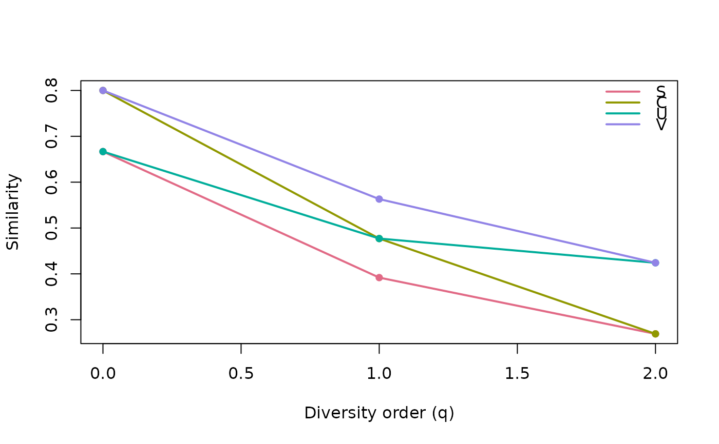
Compute overall similarity metrics from the Hill-number beta diversity
(Chiu et al. 2014). These are 1 - the dissimilarities from hilldiss().
Arguments
- data
A count table (taxa x samples) or a supported object; a single sample is not meaningful for partitioning.
- q
Numeric vector of diversity orders (>= 0). Defaults to
c(0, 1, 2)(richness, Shannon, Simpson).- metric
Dissimilarity metric(s) to return, any of
"S","C","U","V". Defaults to all four.- tree
A phylogenetic tree of class
phylowhose tip labels match the taxa indata.- dist
A functional distance matrix (or
dist) over the taxa.- tau
Optional functional distance threshold. Defaults to
max(dist).- type
Diversity type:
"auto"(default) infers it from the inputs (counts only -> neutral,+tree-> phylogenetic,+dist-> functional); an explicit"neutral","phylogenetic"or"functional"asserts the type and is validated against the inputs (e.g."phylogenetic"requires atree;"neutral"ignores any tree/dist carried by the object).- out
Output shape:
"tibble"(default) returns a long-formatdata.framewith columnsq,metric,value;"matrix"returns the legacy matrix (orders in rows, metrics in columns, dropped to a vector for a single metric).
Value
A long-format data.frame of class hill_similarity (default, with
a plot() method), or a matrix/vector of similarities when
out = "matrix".
Examples
counts <- matrix(c(10, 0, 5, 2, 8, 1), nrow = 3,
                 dimnames = list(c("t1", "t2", "t3"), c("s1", "s2")))
hillsim(counts)
#> similarity from neutral Hill numbers of "q0", "q1", and "q2".
#> <hilldiv3 result: neutral>
#> 12 rows x 3 cols
#>
#>    q metric     value
#> 1  0      S 0.6666667
#> 2  1      S 0.3918610
#> 3  2      S 0.2691680
#> 4  0      C 0.8000000
#> 5  1      C 0.4770152
#> 6  2      C 0.2691680
#> 7  0      U 0.6666667
#> 8  1      U 0.4770152
#> 9  2      U 0.4241645
#> 10 0      V 0.8000000
#> 11 1      V 0.5630749
#> 12 2      V 0.4241645
plot(hillsim(counts))
#> similarity from neutral Hill numbers of "q0", "q1", and "q2".