Partitioning and (dis)similarity • hilldiv3

library(hilldiv3)

Measuring how different samples are from one another is a separate question from how diverse each one is. The classic way to connect the two uses three quantities (Whittaker’s alpha/beta/gamma):

alpha — the diversity within a typical single sample;
gamma — the diversity of all samples pooled together;
beta — how much the samples differ from one another, obtained from the other two.

hilldiv3 computes this split by partitioning gamma into an alpha and a beta component, then (optionally) converting beta into bounded (dis)similarity metrics that are easy to compare across studies. All of this works for neutral, phylogenetic and functional diversity — just add a tree or dist as in the diversity-types article.

counts <- matrix(
  c(10, 0, 5,
     2, 8, 1,
     3, 4, 0,
     6, 2, 7),
  nrow = 3,
  dimnames = list(c("t1", "t2", "t3"), c("s1", "s2", "s3", "s4"))
)

Alpha, gamma and beta

hillpart() returns the three components per diversity order:

hillpart(counts)
#> Partitioning neutral Hill numbers of "q0", "q1", and
#> "q2".
#> <hilldiv3 result: neutral>
#> 9 rows x 3 cols
#> 
#>   q component    value
#> 1 0     alpha 2.500000
#> 2 1     alpha 2.154269
#> 3 2     alpha 1.968927
#> 4 0     gamma 3.000000
#> 5 1     gamma 2.905735
#> 6 2     gamma 2.828374
#> 7 0      beta 1.200000
#> 8 1      beta 1.348827
#> 9 2      beta 1.436505

alpha — the effective diversity of a typical single sample.
gamma — the effective diversity of all samples pooled.
beta — gamma / alpha, the effective number of distinct communities. It ranges from 1 (all samples identical) to N (all samples completely distinct), where N is the number of samples.

Beta is the multiplicative decomposition of Jost (2007): it is independent of alpha, which is what makes it comparable across datasets with different richness.

Multi-scale (hierarchical) partitioning

Real sampling designs are usually nested: replicates within sites, sites within regions, regions within a study. A single alpha/beta split throws that structure away — it cannot tell you whether turnover happens between nearby replicates or between distant regions. hillpart() solves this with a hierarchy formula that decomposes gamma into one beta per hierarchical level, so you can see at which spatial (or temporal, or organisational) scale diversity actually turns over.

Supply the nesting as a one-sided formula, coarsest to finest, plus a metadata table giving each sample’s group memberships:

set.seed(1)
tab <- matrix(rpois(12 * 8, 5), nrow = 12,
              dimnames = list(paste0("t", 1:12), paste0("s", 1:8)))
md <- data.frame(
  region = rep(c("N", "S"), each = 4),
  site   = rep(c("a", "b", "c", "d"), each = 2),
  row.names = paste0("s", 1:8)
)

hillpart(tab, hierarchy = ~ region / site, metadata = md)
#> Partitioning neutral Hill numbers across scales "sample < site < region <
#> total".
#> <hilldiv3 result: neutral>
#> 12 rows x 5 cols
#> 
#>    q  scale n_units diversity     beta
#> 1  0 sample       8  12.00000       NA
#> 2  0   site       4  12.00000 1.000000
#> 3  0 region       2  12.00000 1.000000
#> 4  0  total       1  12.00000 1.000000
#> 5  1 sample       8  11.11495       NA
#> 6  1   site       4  11.60076 1.043708
#> 7  1 region       2  11.77266 1.014817
#> 8  1  total       1  11.95901 1.015829
#> 9  2 sample       8  10.47242       NA
#> 10 2   site       4  11.24852 1.074109
#> 11 2 region       2  11.56260 1.027923
#> 12 2  total       1  11.92231 1.031110

The result is one row per (q, scale), finest (sample) to coarsest (total):

diversity is the effective diversity at that scale (A_k): the per-sample alpha at sample, the pooled gamma at total, interpolating in between.
beta is the turnover gained at that scale, A_k / A_{k-1} — e.g. the site beta is turnover among samples within a site, the region beta among sites within a region, the total beta among regions.
n_units is how many units exist at that scale (8 samples → 4 sites → 2 regions → 1 total).

The betas multiply back to the overall beta exactly:

${}^qD_\gamma \;=\; {}^qD_\alpha \,\cdot\, \prod_k \beta_k .$

This telescoping identity is guaranteed by construction (and checked in the package tests), so a hierarchical run is always consistent with the plain hillpart() alpha and gamma. Arbitrarily deep hierarchies work — just chain more terms, e.g. ~ study / region / site. The out = "matrix" form returns the same information as alpha, one beta_<level> column per transition, and gamma.

How it works (and what it assumes)

Advanced — skip on a first read. The formula below explains why the betas behave well; you do not need it to use hillpart(). The practical takeaways are the bullet points on assumptions that follow it.

All three diversity types share one construction under global equal sample weighting (every sample weighted 1/n). Each scale’s diversity is Jost’s (2007) weighted alpha,

$A_k \;=\; \frac{\left(\sum_{u,i} w_i\,(m_{u,i}/C)^q\right)^{1/(1-q)}} {\left(\sum_{u} (n_u/n)^q\right)^{1/(1-q)}},$

where units $u$ pool $n_u$ of the $n$ samples, $m_{u,i}=\sum_{j\in u} c_{ij}$ is the pooled contribution of feature $i$ , $w_i$ is a per-feature measure, and $C$ a grand-total normaliser. The three types differ only in those pieces: neutral uses taxa with measure $1$ and $C=n$ ; phylogenetic uses branches with measure $L_i$ (branch length) and $C=T_+=\sum_j T_j$ (summed tree depth); functional uses taxa with measure $v_i$ (attribute contribution at threshold tau) and $C=n_+$ (total count). The denominator is the numbers-equivalent of the unit weights, which is exactly what keeps every $\beta_k \ge 1$ and independent of $A$ .

Phylogenetic and functional hierarchical partitioning simply add a tree or dist, as everywhere else in hilldiv3:

hillpart(tab, hierarchy = ~ region / site, metadata = md, tree = my_tree)
hillpart(tab, hierarchy = ~ region / site, metadata = md, dist = my_dist)

Limitations and assumptions — worth knowing before interpreting the betas:

Equal per-sample weighting only. Units are weighted by their sample count (n_u / n), not by abundance or sampling effort. This is the choice that makes every beta independent of alpha for all q (Jost 2007); unequal weighting breaks that independence for q ≠ 1 and is not offered.
Phylogenetic: one shared tree depth across scales. Alpha and gamma are reported in effective-branch-length (PD) units and share a single mean depth T_+ over all scales, which is what lets the betas telescope. For ultrametric trees the finest alpha equals the single-level phylogenetic hillpart() alpha exactly; for non-ultrametric trees the chain still telescopes, but the shared T_+ makes the per-scale PD values depth-pooled rather than strictly per-sample — prefer ultrametric (time-calibrated) trees here.
Functional: one shared tau and v_i across scales. The distance threshold is capped once over the whole table and the attribute contributions v_i are computed once from the fully pooled data, so they stay constant across scales (a prerequisite for telescoping). A per-subset tau is therefore not meaningful in a hierarchical run.
Hierarchical output is not (yet) wired into hilldiss()/hillsim() or hillpair(). Those convert a single beta to bounded (dis)similarity; the per-level rescaling of a nested beta chain is left for future work.

This nested multiplicative decomposition across neutral, phylogenetic and functional Hill numbers in one engine is, to our knowledge, not available in other packages; it generalises the single-level partition above rather than replacing it.

From beta to (dis)similarity

Beta lives on [1, N], which is awkward to compare across studies with different sample counts. hilldiss() and hillsim() rescale it to [0, 1] using the four overlap measures of Chiu et al. (2014):

Code	Measure	Type
`S`	Sorensen-type	local overlap, occurrence-flavoured
`C`	Jaccard-type (Morisita-Horn at `q = 2`)	local overlap, abundance-flavoured
`U`	one-minus regional overlap	regional
`V`	homogeneity / Sorensen complement	regional

hilldiss(counts)            # dissimilarities, one column per metric
#> dissimilarity from neutral Hill numbers of "q0", "q1",
#> and "q2".
#> <hilldiv3 result: neutral>
#> 12 rows x 3 cols
#> 
#>    q metric      value
#> 1  0      S 0.22222222
#> 2  1      S 0.34481987
#> 3  2      S 0.40515478
#> 4  0      C 0.06666667
#> 5  1      C 0.21585249
#> 6  2      C 0.40515478
#> 7  0      U 0.22222222
#> 8  1      U 0.21585249
#> 9  2      U 0.14550174
#> 10 0      V 0.06666667
#> 11 1      V 0.11627556
#> 12 2      V 0.14550174
hillsim(counts)             # similarities = 1 - dissimilarity
#> similarity from neutral Hill numbers of "q0", "q1", and
#> "q2".
#> <hilldiv3 result: neutral>
#> 12 rows x 3 cols
#> 
#>    q metric     value
#> 1  0      S 0.7777778
#> 2  1      S 0.6551801
#> 3  2      S 0.5948452
#> 4  0      C 0.9333333
#> 5  1      C 0.7841475
#> 6  2      C 0.5948452
#> 7  0      U 0.7777778
#> 8  1      U 0.7841475
#> 9  2      U 0.8544983
#> 10 0      V 0.9333333
#> 11 1      V 0.8837244
#> 12 2      V 0.8544983

Request a single metric and order to get a plain matrix slice:

hilldiss(counts, q = 1, metric = "C")
#> dissimilarity from neutral Hill numbers of "q1".
#> <hilldiv3 result: neutral>
#> 1 rows x 3 cols
#> 
#>   q metric     value
#> 1 1      C 0.2158525

The choice of q matters as much as the metric: q = 0 weights presence/ absence (turnover of rare taxa), while q = 2 reflects shifts among dominant taxa.

Pairwise dissimilarity for ordination

hilldiss() summarises all samples at once. To compare samples two-by-two — the input ordination methods expect — use hillpair(), which returns a dist object (or a long tibble):

d <- hillpair(counts, q = 1, metric = "C")
#> Computing neutral pairwise dissimilarity for 6 sample pairs.
d
#>            s1         s2         s3
#> s2 0.52298484                      
#> s3 0.47119926 0.08924381           
#> s4 0.09902103 0.29281463 0.33948330

That dist drops straight into ordination and clustering:

pcoa <- cmdscale(d, k = 2)
plot(pcoa, type = "n", xlab = "PCoA 1", ylab = "PCoA 2")
text(pcoa, labels = rownames(pcoa))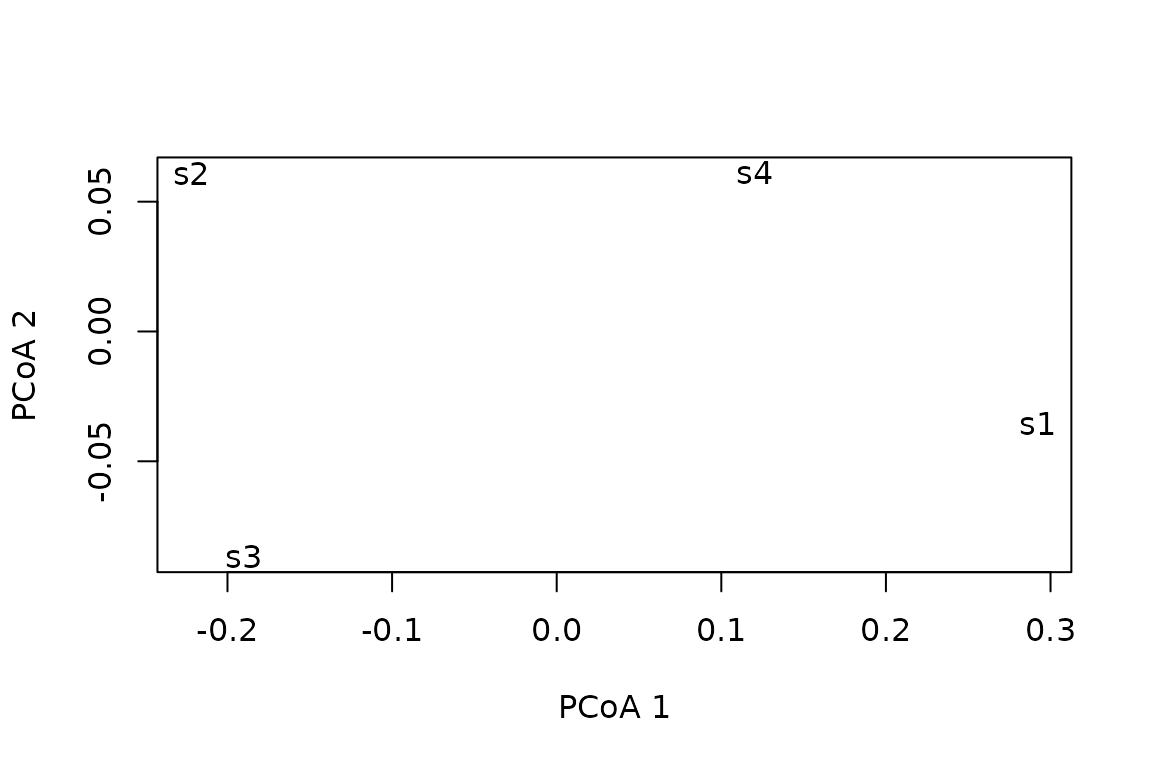

PCoA of pairwise Hill-number dissimilarities

Ask for several orders/metrics at once and you get a named list of dist objects (e.g. q0S, q1C):

ds <- hillpair(counts, q = c(0, 2), metric = c("C", "U"))
#> Computing neutral pairwise dissimilarity for 6 sample pairs.
names(ds)
#> [1] "q0C" "q2C" "q0U" "q2U"

Or a tidy long table, convenient for ggplot2 or dplyr:

head(hillpair(counts, q = 1, metric = "C", out = "tibble"))
#> Computing neutral pairwise dissimilarity for 6 sample pairs.
#>   first second q metric      value
#> 1    s1     s2 1      C 0.52298484
#> 2    s1     s3 1      C 0.47119926
#> 3    s1     s4 1      C 0.09902103
#> 4    s2     s3 1      C 0.08924381
#> 5    s2     s4 1      C 0.29281463
#> 6    s3     s4 1      C 0.33948330

Larger datasets

hillpair() computes every pair through the same partitioning engine, so cost grows with the number of pairs. For many samples, run pairs in parallel by setting parallel = TRUE with a future plan and the furrr package installed:

library(future)
plan(multisession)
hillpair(counts, q = 1, metric = "C", parallel = TRUE)

Contrasts with other packages

Advanced — skip on a first read. This section is for users coming from other Hill-number tools who want to reconcile differing numbers. Newcomers can safely move on.

hillR and hilldiv2 also split Hill numbers into alpha, gamma and beta. For neutral and phylogenetic diversity their partitions match hilldiv3 to numerical precision: hilldiv2::hillpart(), hillR::hill_taxa_parti() and hillR::hill_phylo_parti() return the same alpha, gamma and beta as hillpart(). The functional partition is where they part ways — and, as in the diversity types article, these are convention differences, not bugs.

`hillR::hill_func_parti`

Three choices stack up, which is why the numbers look unrelated (≈1.5 vs several thousand) rather than merely rescaled:

What is reported. hilldiv3 returns the functional Hill number qD — an effective number of functionally distinct species, bounded in [1, S] and in the same currency as its neutral and phylogenetic output. hill_func_parti() returns the functional attribute diversity FD = qD^2 * Q (where Q is Rao’s quadratic entropy); at q = 0 this is sum(d_ij), the total pairwise distance (Walker’s FAD). The squaring and the Q factor account for most of the apparent gap.
The distance threshold tau. hilldiv3 uses tau = max(d_ij) by default; hill_func_parti() fixes tau = Q (≈ the abundance-weighted mean distance). A smaller tau makes species look more distinct and inflates qD, so the threshold alone shifts the effective count several-fold. hilldiv3 exposes tau as an argument, so you can match either convention — or, as Chiu, Jost & Chao (2014) recommend, profile diversity across a range of tau.
The scale of beta. Because FD squares the Hill number, hillR’s functional beta FD_gamma / FD_alpha equals (qD_gamma / qD_alpha)^2 and lives in [1, N^2]. hilldiv3’s functional beta is the Hill ratio qD_gamma / qD_alpha in [1, N], directly comparable to its own neutral and phylogenetic betas. A hillR functional beta of 1.6 is therefore not on the same scale as a taxonomic beta of 1.6.

hilldiv2::hillpart() shares hilldiv3’s conventions exactly — the same tau = max(d_ij) threshold and the same functional Hill number qD — so its functional partition matches hilldiv3 to machine precision.

traits <- data.frame(body_size = c(1, 5, 9), row.names = rownames(counts))
d <- dist(traits)

# hilldiv3 reports the functional Hill number qD (effective number of species).
hillpart(counts, q = c(0, 1, 2), dist = d)

# hillR reports FD = qD^2 * Q (a different scale); it fixes tau = Rao's Q.
hillR::hill_func_parti(t(counts), traits, q = 1)

Nested hierarchies

The multi-scale partitioning above has no equivalent in either package: neither hillR nor hilldiv2 accepts a nested hierarchy, so telescoping gamma = alpha * prod(beta) across region/site levels is specific to hilldiv3.

Want to match	Use in `hilldiv3`
`hillR::hill_taxa_parti()` (neutral)	`hillpart()` (exact)
`hillR::hill_phylo_parti()` (phylogenetic)	`hillpart(tree = ...)` (exact)
`hillR::hill_func_parti()` (functional)	no exact match — it reports `FD`, not `qD`; set `tau = Q` to align the threshold
`hilldiv2::hillpart()` (any type)	`hillpart()` (exact)

In short: when functional partitions diverge, check (1) whether the other package reports an effective number (qD) or attribute diversity (FD), and (2) which tau it uses. hilldiv3 keeps functional diversity in the same effective-number currency as its neutral and phylogenetic facets, and makes tau explicit.

References

Jost, L. (2007). Partitioning diversity into independent alpha and beta components. Ecology, 88, 2427–2439.
Chiu, C.-H., Jost, L. & Chao, A. (2014). Phylogenetic beta diversity, similarity, and differentiation measures based on Hill numbers. Ecological Monographs, 84, 21–44.