Case 1: Dietary niches of insectivorous bats • hilldiv3

library(hilldiv3)
library(ggplot2)

theme_set(theme_bw(base_size = 12) +
            theme(panel.grid.minor = element_blank(),
                  legend.position = "top"))

# hilldiv3 results are long-format data.frame subclasses; drop the class so
# base `$<-` / `rbind` (and ggplot2) work without coercion.
as_df <- function(x) { class(x) <- "data.frame"; x }
pal <- c(forest = "#2E7D32", farmland = "#C9A227")

New to Hill numbers? This is a complete worked example. If terms like diversity order q, alpha/beta diversity or phylogenetic diversity are unfamiliar, start with the Getting started guide and the Diversity types article, then come back here.

Dietary metabarcoding turns faecal or guano samples into a count table of prey amplicon sequence variants (ASVs), and a question that immediately follows is how diverse, and how different, are the diets of the animals we sampled? Because the prey of a predator are an arbitrary slice of the tree of life, counting ASVs alone can mislead: a bat that takes twenty species of moth has a taxon-rich but phylogenetically narrow diet, whereas a bat that takes a beetle, a fly and a true bug eats fewer taxa spread across far more of the insect phylogeny. hilldiv3 makes both readings available from the same call, and lets us ask at which level of a nested sampling design dietary turnover actually occurs.

The data

We use a simulated guano-metabarcoding design: 50 insect-prey ASVs detected across 30 individual bats, nested as 5 individuals × 3 roosts × 2 contrasting foraging habitats (forest vs. farmland). Prey ASVs belong to four insect orders, and their phylogeny has shallow within-order clades on a deep order-level backbone. Forest bats are specialists, concentrating on a single dominant moth (Lepidoptera) clade; farmland bats are generalists spread evenly across Diptera, Coleoptera and Hemiptera.

The full simulation ships with the package (and is reproducible); we simply source it here to obtain a count table (bat_counts), a prey phylogeny (bat_tree) and a sample-design table (bat_metadata).

data_candidates <- c(
  file.path("inst", "manuscript", "data-bat-diet.R"),
  file.path("..", "inst", "manuscript", "data-bat-diet.R"),
  file.path("..", "..", "inst", "manuscript", "data-bat-diet.R"),
  system.file("manuscript", "data-bat-diet.R", package = "hilldiv3")
)
data_candidates <- data_candidates[nzchar(data_candidates)]
data_path <- data_candidates[file.exists(data_candidates)][[1]]

sim <- source(data_path)$value
bat_counts   <- sim$counts
bat_tree     <- sim$tree
bat_metadata <- sim$metadata

dim(bat_counts)                 # 50 prey ASVs x 30 bats
#> [1] 50 30
range(colSums(bat_counts > 0))  # per-sample prey richness
#> [1] 12 25
head(bat_metadata)
#>       habitat  roost   bat
#> bat01  forest roost1 bat01
#> bat02  forest roost1 bat02
#> bat03  forest roost1 bat03
#> bat04  forest roost1 bat04
#> bat05  forest roost1 bat05
#> bat06  forest roost2 bat06

hab <- function(s) bat_metadata$habitat[match(s, bat_metadata$bat)]

Neutral and phylogenetic diversity from one interface

hilldiv() returns Hill numbers per sample at diversity orders q = 0 (richness), q = 1 (Shannon) and q = 2 (Simpson). The computation is cumulative: adding tree = returns neutral and phylogenetic diversity together in one tibble, tagged by a type column (type = keeps just one).

# A single call with `tree =` returns both flavours, tagged by `type`.
labs <- c(neutral = "Neutral (qD)", phylogenetic = "Phylogenetic (qPD)")
alpha <- as_df(hilldiv(bat_counts, q = c(0, 1, 2), tree = bat_tree))
alpha$flavour <- factor(labs[alpha$type], labs)
alpha$habitat <- hab(alpha$sample)

aggregate(value ~ flavour + q + habitat, alpha, function(x) round(mean(x), 2))
#>               flavour q  habitat value
#> 1        Neutral (qD) 0 farmland 19.20
#> 2  Phylogenetic (qPD) 0 farmland  2.95
#> 3        Neutral (qD) 1 farmland 14.69
#> 4  Phylogenetic (qPD) 1 farmland  1.85
#> 5        Neutral (qD) 2 farmland 12.28
#> 6  Phylogenetic (qPD) 2 farmland  1.51
#> 7        Neutral (qD) 0   forest 16.47
#> 8  Phylogenetic (qPD) 0   forest  2.83
#> 9        Neutral (qD) 1   forest  8.38
#> 10 Phylogenetic (qPD) 1   forest  1.72
#> 11       Neutral (qD) 2   forest  6.00
#> 12 Phylogenetic (qPD) 2   forest  1.46

ggplot(alpha, aes(factor(q), value, fill = habitat)) +
  geom_boxplot(outlier.size = 0.6, width = 0.7) +
  facet_wrap(~ flavour, scales = "free_y") +
  scale_fill_manual(values = pal, name = NULL) +
  labs(x = "Diversity order (q)", y = "Effective number of prey lineages")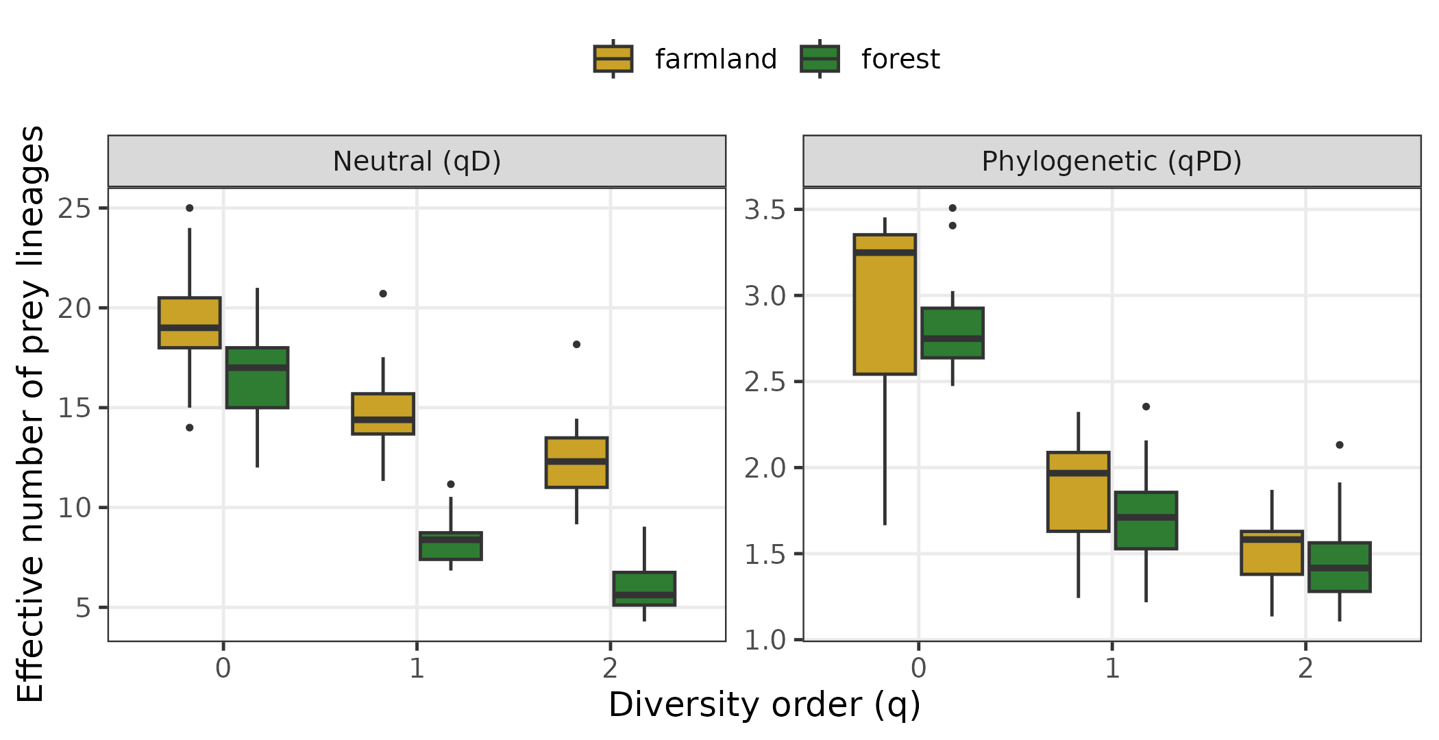

Neutral and phylogenetic alpha diversity by habitat across q

Forest specialists and farmland generalists differ only modestly in prey richness (q = 0), but the gap widens sharply at higher q: at q = 2 the forest diet collapses to an effective ~6 prey ASVs against ~12 in farmland, because a few dominant moths carry most of the forest reads. The phylogenetic numbers show that the farmland diet is also consistently broader across the insect phylogeny — the generalists span more of the prey tree of life even where their taxon counts are similar.

Diversity profiles make the dominance structure explicit

Reading diversity at a single q can mislead; a diversity profile, hillprof(), traces qD continuously and exposes the whole evenness structure in one curve.

prof <- as_df(hillprof(bat_counts, q = seq(0, 3, by = 0.1)))
prof$habitat <- hab(prof$sample)
prof_mean <- aggregate(value ~ q + habitat, prof, mean)

ggplot(prof, aes(q, value, group = sample, colour = habitat)) +
  geom_line(alpha = 0.25, linewidth = 0.3) +
  geom_line(data = prof_mean, aes(group = habitat), linewidth = 1.3) +
  scale_colour_manual(values = pal, name = NULL) +
  labs(x = "Diversity order (q)", y = "Neutral diversity (qD)")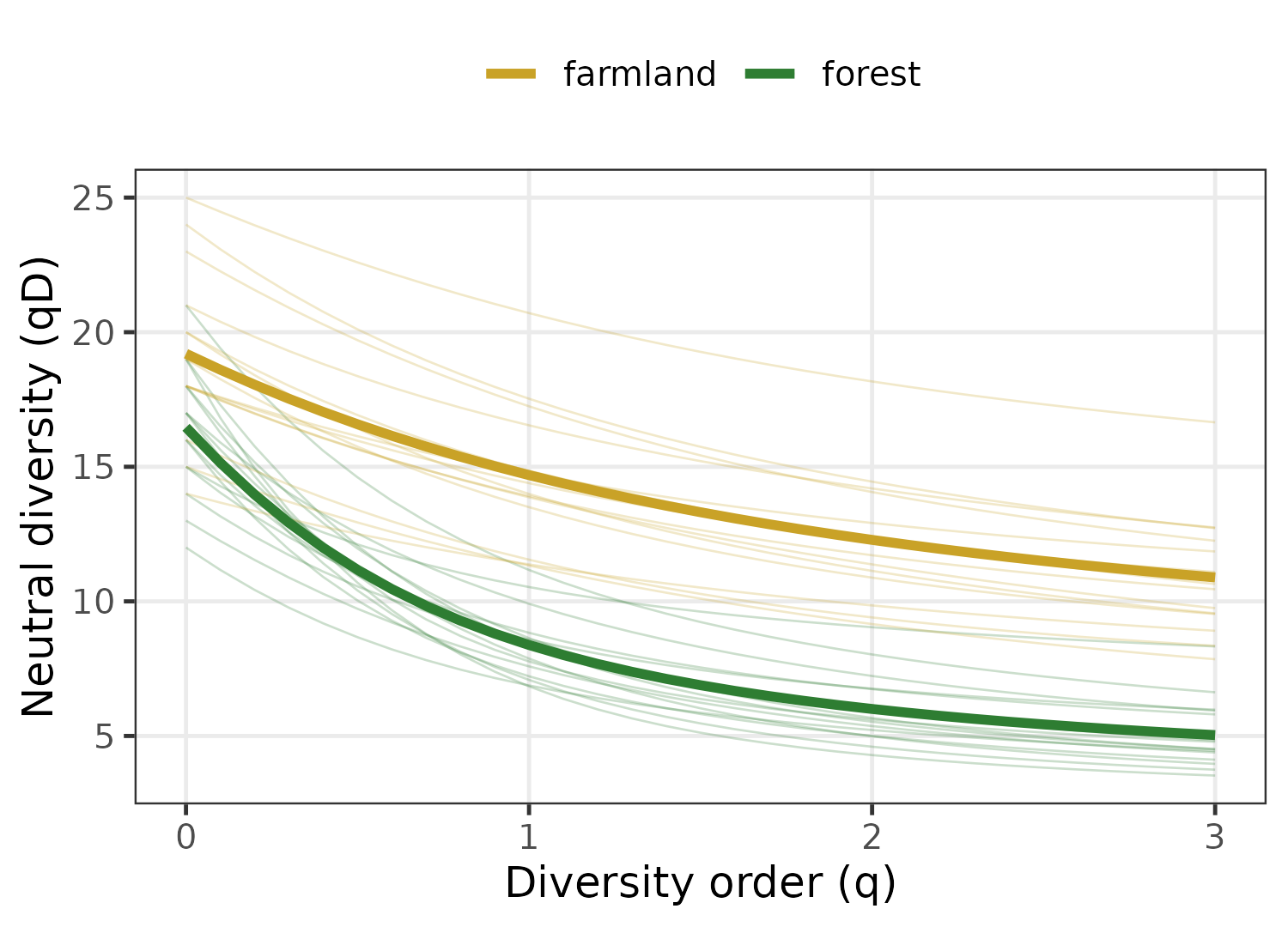

The forest profiles fall away more steeply and sit lower — the signature of a few dominant prey — while the farmland profiles decline gently from a higher richness, the signature of a more even diet. hilleven() condenses this into a single number:

even <- as_df(hilleven(bat_counts, q = 2))
even$habitat <- hab(even$sample)
aggregate(value ~ habitat, even, function(x) round(mean(x), 3))
#>    habitat value
#> 1 farmland 0.640
#> 2   forest 0.372

The mean q = 2 evenness is far lower in forest than in farmland, confirming that forest diets are dominated by a handful of moth ASVs.

At which scale does the diet turn over?

A nested design asks a question a single alpha/beta split cannot answer: does diet vary mostly between individual bats, between roosts, or between habitats? hillpart() answers it directly with a one-sided hierarchy formula, decomposing the pooled (gamma) diversity into one beta per hierarchical level. Each beta is the turnover gained at that scale, and the chain telescopes exactly (gamma = alpha_finest × ∏ beta).

hier_n <- hillpart(bat_counts, q = c(0, 1, 2),
                   hierarchy = ~ habitat / roost, metadata = bat_metadata)
hier_p <- hillpart(bat_counts, q = c(0, 1, 2), tree = bat_tree,
                   hierarchy = ~ habitat / roost, metadata = bat_metadata)
hier_p
#> <hilldiv3 result: phylogenetic>
#> 12 rows x 5 cols
#> 
#>    q   scale n_units diversity     beta
#> 1  0  sample      30  2.889998       NA
#> 2  0   roost       6  3.688281 1.276222
#> 3  0 habitat       2  3.905978 1.059024
#> 4  0   total       1  4.170406 1.067698
#> 5  1  sample      30  1.757890       NA
#> 6  1   roost       6  1.881011 1.070039
#> 7  1 habitat       2  1.910385 1.015616
#> 8  1   total       1  2.729837 1.428946
#> 9  2  sample      30  1.447888       NA
#> 10 2   roost       6  1.484669 1.025403
#> 11 2 habitat       2  1.496183 1.007755
#> 12 2   total       1  2.387101 1.595461

beta_n <- as_df(hier_n); beta_p <- as_df(hier_p)
beta_n <- beta_n[beta_n$scale != "sample", ]; beta_n$flavour <- "Neutral"
beta_p <- beta_p[beta_p$scale != "sample", ]; beta_p$flavour <- "Phylogenetic"
betas <- rbind(beta_n, beta_p)
betas$scale <- factor(betas$scale, c("roost", "habitat", "total"),
                      labels = c("among individuals\n(within roost)",
                                 "among roosts\n(within habitat)",
                                 "among habitats"))

ggplot(betas, aes(scale, beta, fill = factor(q))) +
  geom_col(position = position_dodge(0.8), width = 0.7) +
  facet_wrap(~ flavour) +
  geom_hline(yintercept = 1, linetype = 2, colour = "grey40") +
  scale_fill_brewer(palette = "Blues", name = "q") +
  labs(x = NULL, y = expression("Turnover gained at scale (" * beta[k] * ")"))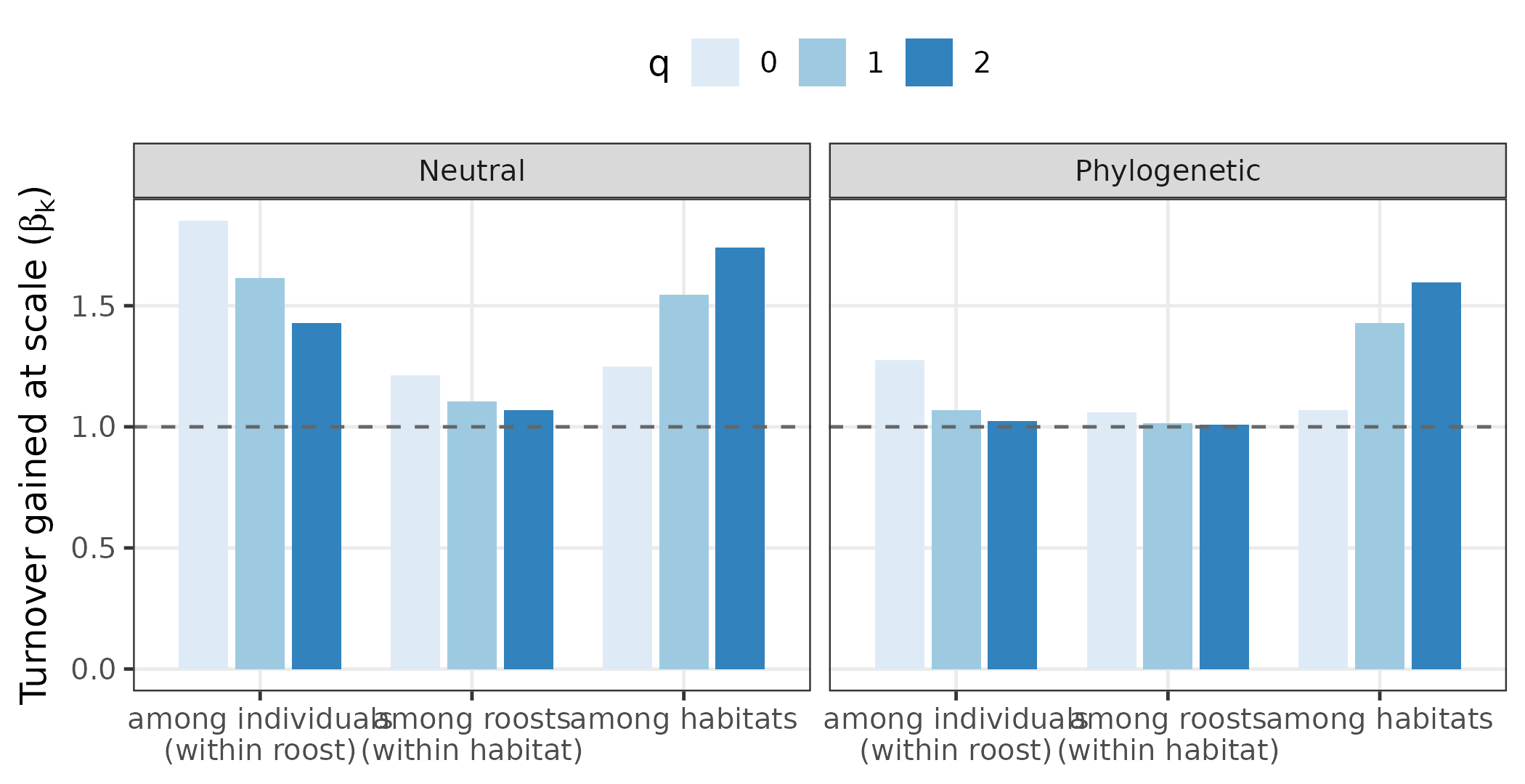

Turnover gained at each nested scale, neutral versus phylogenetic

The two flavours localise turnover to different scales. Neutral turnover is split between individuals and habitats: bats sample different exact prey ASVs from one mouthful to the next, and the two habitats offer different prey. But phylogenetic turnover is concentrated almost entirely between habitats and is negligible within them: individuals in the same habitat eat phylogenetically interchangeable prey, while the forest and farmland diets are drawn from genuinely different parts of the insect tree. This neutral-vs-phylogenetic, scale-resolved contrast — available across all three diversity types from one engine — is unique to hilldiv3.

Summary

From a single ASV table and a prey tree, hilldiv3 delivered: per-sample neutral and phylogenetic Hill numbers (hilldiv()), full diversity profiles (hillprof()) and evenness (hilleven()), and a scale-resolved nested partition of turnover under both flavours (hillpart() with a hierarchy formula) — a complete dietary-diversity analysis through one consistent interface. The neutral-versus-phylogenetic contrast, resolved across the whole diversity profile and across every level of the nested design, is what lets a single study say not just how much diets differ but in what currency and at which scale.

References

Hill, M.O. (1973). Diversity and evenness. Ecology, 54, 427–432.
Jost, L. (2007). Partitioning diversity into independent alpha and beta components. Ecology, 88, 2427–2439.
Alberdi, A. & Gilbert, M.T.P. (2019). A guide to the application of Hill numbers to DNA-based diversity analyses. Mol. Ecol. Resour., 19, 804–817.