Profiles, evenness and redundancy

library(hilldiv3)

Beyond a single diversity number, hilldiv3 offers three diagnostics that describe the shape of a community: profiles (how diversity changes with the order q), evenness (how equitably abundance is spread), and redundancy (how much phylogenetic/functional structure is duplicated).

counts <- matrix(
  c(10, 0, 5,
     2, 8, 1,
     3, 4, 0,
     6, 2, 7),
  nrow = 3,
  dimnames = list(c("t1", "t2", "t3"), c("s1", "s2", "s3", "s4"))
)
tree <- ape::read.tree(text = "((t1:1,t2:1):1,t3:2);")

Diversity profiles

A single q can mislead: two samples can have identical richness but very different Shannon or Simpson diversity, and their ranking can even flip as q increases. A profile plots Hill numbers across a continuous sweep of q, making the full picture visible. hillprof() evaluates a fine grid of orders (0 to 3 by default):

prof <- hillprof(counts)
#> Computing neutral diversity profile over 31 orders.
head(prof)
#> <hilldiv3 result: neutral>
#> 6 rows x 3 cols
#> 
#>     q sample    value
#> 1 0.0     s1 2.000000
#> 2 0.1     s1 1.988282
#> 3 0.2     s1 1.976692
#> 4 0.3     s1 1.965243
#> 5 0.4     s1 1.953945
#> 6 0.5     s1 1.942809

The result is a tidy long-format object with a ready-made plot method — one declining curve per sample:

plot(prof)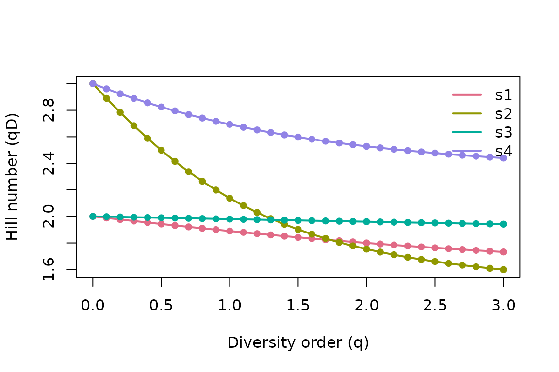

How to read it:

• The height at q = 0 is richness; the height as q → ∞ reflects dominance.
• A flat curve means an even community (diversity barely changes with q); a steep curve means a few taxa dominate.
• If two curves cross, neither sample is unambiguously more diverse — the answer depends on how much you weight rare taxa.

Profiles work for phylogenetic and functional diversity too, and you can grab a matrix instead of the tidy form (samples in rows, diversity orders in columns):

phylo_prof <- hillprof(counts, tree = tree)
#> Computing phylogenetic diversity profile over 31 orders.
mat <- hillprof(counts, out = "matrix")
#> Computing neutral diversity profile over 31 orders.
mat[, 1:3]
#>    q0     q0.1     q0.2
#> s1  2 1.988282 1.976692
#> s2  3 2.889634 2.783926
#> s3  2 1.997940 1.995884
#> s4  3 2.961206 2.924319

Evenness

Evenness asks how equitably abundance is distributed, independent of richness. hilleven() expresses it as the ratio of diversity of order q to richness (qD / 0D), which is bounded in [0, 1]: 1 is perfectly even, lower values mean stronger dominance.

hilleven(counts)
#> Computing neutral evenness of "q1" and "q2".
#> <hilldiv3 result: neutral>
#> 8 rows x 3 cols
#> 
#>   q sample     value
#> 1 1     s1 0.9449408
#> 2 2     s1 0.9000000
#> 3 1     s2 0.7124362
#> 4 2     s2 0.5845411
#> 5 1     s3 0.9898132
#> 6 2     s3 0.9800000
#> 7 1     s4 0.8978279
#> 8 2     s4 0.8426966

This is exactly the normalised height of the diversity profile — a single sample’s profile flatness summarised as a number. Reading down a column tells you how dominated each sample is; s2 here is the least even.

Redundancy

Neutral diversity counts taxa; phylogenetic and functional diversity count distinct lineages or trait combinations. When taxa are closely related or functionally similar, much of the neutral diversity is redundant — losing a taxon costs little unique phylogenetic/functional diversity.

hillred() quantifies this by fitting the saturating relationship between neutral diversity (x) and phylogenetic/functional diversity (y) across samples, y = -a · 2^(-x / b) + c, and summarising redundancy as 1 - b / max(x). It therefore needs a tree or dist, and several samples spanning a range of neutral diversity to fit the curve. The three-taxon toy matrix above is too small, so here we use the bundled gut_* data (24 taxa across 12 gut microbiome samples):

hillred(gut_counts, q = c(1, 2), tree = gut_tree)
#> <hilldiv3 result: phylogenetic>
#> 2 rows x 5 cols
#> 
#>   q redundancy         a        b        c
#> 1 1  0.9022283 21.932974 1.533208 2.187965
#> 2 2  0.9098232  4.175493 1.166743 1.665108

The returned table has the redundancy summary plus the fitted a, b, c coefficients per order. Values near 1 mean the assemblage is highly redundant (taxa are phylogenetically/functionally interchangeable); values near 0 mean each taxon contributes largely unique diversity.

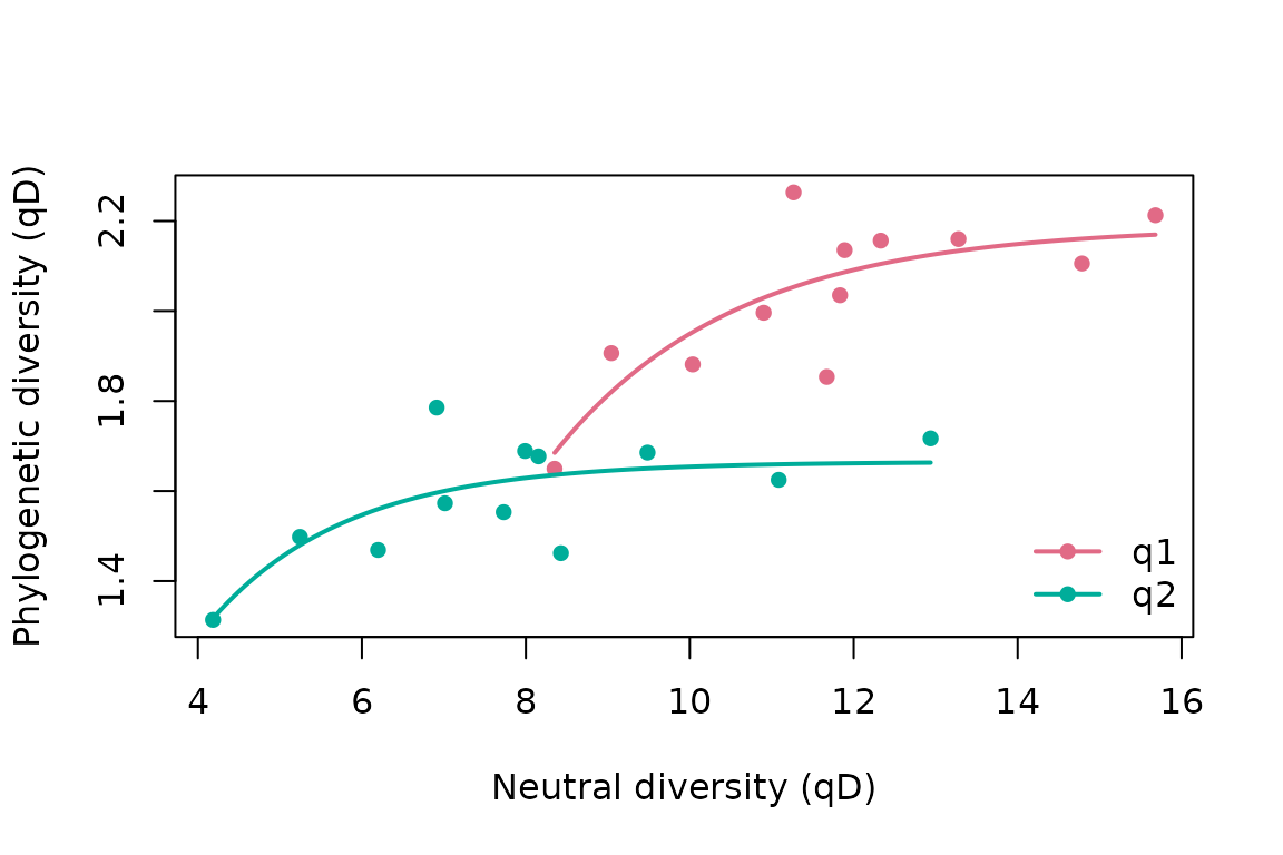
Like the profile, the result has a ready-made plot() method. It draws the fit behind the redundancy number: each sample’s neutral diversity against its phylogenetic/functional diversity, with the fitted saturating curve per order. A curve that bends early and plateaus signals high redundancy.

red <- hillred(gut_counts, q = c(1, 2), tree = gut_tree)
plot(red)

Note. Redundancy is a curve fit across samples, so it needs several samples spanning a range of neutral diversity. Orders where that spread is missing return NA with a warning rather than a number. In particular, richness (q = 0) often cannot be fit on well-sampled data: when nearly every sample contains nearly every taxon, richness barely varies across samples and the curve’s rate is unidentifiable — which is why the example above uses q = 1 and q = 2.

References

• Hill, M.O. (1973). Diversity and evenness. Ecology, 54, 427–432.
• Chao, A., Chiu, C.-H. & Jost, L. (2010). Phylogenetic diversity measures based on Hill numbers. Phil. Trans. R. Soc. B, 365, 3599–3609.
• Alberdi, A. & Gilbert, M.T.P. (2019). A guide to the application of Hill numbers to DNA-based diversity analyses. Mol. Ecol. Resour., 19, 804–817.