Case 2: Three faces of diversity in a gut microbiome

library(hilldiv3)
library(ggplot2)

theme_set(theme_bw(base_size = 12) +
            theme(panel.grid.minor = element_blank(),
                  legend.position = "top"))

# hilldiv3 results are long-format data.frame subclasses; drop the class so
# base `$<-` / `rbind` (and ggplot2) work without coercion.
as_df <- function(x) { class(x) <- "data.frame"; x }
pal <- c(control = "#1F77B4", treatment = "#D62728")

New to Hill numbers? This is a complete worked example. If terms like diversity order q, alpha/beta diversity or phylogenetic/functional diversity are unfamiliar, start with the Getting started guide and the Diversity types article, then come back here.

Genome-resolved metagenomics summarises a microbial community as a table of metagenome-assembled genome (MAG) abundances. Each MAG carries two extra layers of information that a raw count ignores: its position on the bacterial phylogeny and its functional attributes (genome size, GC content, oxygen tolerance, encoded capabilities). These layers can move independently: an intervention may reshuffle which organisms — and which lineages — dominate a community while leaving what the community does untouched, if the incoming genomes are functionally equivalent to the ones they replace. hilldiv3 measures all three flavours from the same count table and the same calls, so taxonomic, phylogenetic and functional change can be compared on a common, interpretable scale (effective numbers of lineages) — and, crucially, told apart.

The data

We use the bundled simulated data set: 24 MAGs across 12 host gut samples, split into a control and a treatment group of six. The MAGs fall into two deep bacterial clades, and the intervention swaps which clade dominates: control guts are dominated by clade A, treatment guts by clade B, with taxon richness left untouched. The two clades are functional mirrors of one another — for every genome in one there is a genome in the other with the same trait profile — so a swap that is dramatic phylogenetically is invisible functionally. gut_tree is the genome phylogeny and gut_traits a trait table mixing continuous (genome_size, gc_content), categorical (oxygen) and binary (motility) attributes.

group <- rep(c("control", "treatment"), each = 6)
names(group) <- colnames(gut_counts)
metadata <- data.frame(group = group, row.names = colnames(gut_counts))
grp <- function(s) group[s]

dim(gut_counts)                 # 24 MAGs x 12 samples
#> [1] 24 12
range(colSums(gut_counts > 0))  # per-sample richness (near-constant)
#> [1] 23 24
head(gut_traits)
#>       genome_size gc_content         oxygen motility
#> mag01        1.64      0.343       anaerobe        0
#> mag02        1.97      0.354 microaerophile        1
#> mag03        2.34      0.400    facultative        0
#> mag04        2.75      0.420         aerobe        1
#> mag05        3.20      0.447       anaerobe        0
#> mag06        3.66      0.496 microaerophile        1

traits2dist() turns that mixed trait table into a functional distance with Gower’s coefficient, which handles the different variable types automatically:

fdist <- traits2dist(gut_traits)
range(fdist)
#> [1] 0.0000000 0.9988839

Neutral, phylogenetic and functional diversity from one call

The diversity type follows from what you supply, cumulatively: counts give neutral, tree = adds phylogenetic, dist = adds functional. Supplying both a tree and a distance matrix returns all three at once in a single tibble, with a type column telling them apart (type = restricts the output). The interface never changes.

# One call with both `tree =` and `dist =` returns neutral, phylogenetic and
# functional diversity together, tagged by a `type` column.
labs <- c(neutral = "Neutral (qD)", phylogenetic = "Phylogenetic (qPD)",
          functional = "Functional (qFD)")
alpha <- as_df(hilldiv(gut_counts, q = c(0, 1, 2),
                       tree = gut_tree, dist = fdist))
alpha$flavour <- factor(labs[alpha$type], labs)
alpha$group   <- grp(alpha$sample)

aggregate(value ~ flavour + q + group, alpha, function(x) round(mean(x), 2))
#>               flavour q     group value
#> 1        Neutral (qD) 0   control 23.83
#> 2  Phylogenetic (qPD) 0   control  3.76
#> 3    Functional (qFD) 0   control  1.93
#> 4        Neutral (qD) 1   control 12.25
#> 5  Phylogenetic (qPD) 1   control  2.10
#> 6    Functional (qFD) 1   control  1.90
#> 7        Neutral (qD) 2   control  8.11
#> 8  Phylogenetic (qPD) 2   control  1.64
#> 9    Functional (qFD) 2   control  1.87
#> 10       Neutral (qD) 0 treatment 23.50
#> 11 Phylogenetic (qPD) 0 treatment  3.75
#> 12   Functional (qFD) 0 treatment  1.87
#> 13       Neutral (qD) 1 treatment 11.26
#> 14 Phylogenetic (qPD) 1 treatment  1.96
#> 15   Functional (qFD) 1 treatment  1.85
#> 16       Neutral (qD) 2 treatment  7.78
#> 17 Phylogenetic (qPD) 2 treatment  1.54
#> 18   Functional (qFD) 2 treatment  1.82

ggplot(alpha, aes(factor(q), value, fill = group)) +
  geom_boxplot(outlier.size = 0.6, width = 0.7) +
  facet_wrap(~ flavour, scales = "free_y") +
  scale_fill_manual(values = pal, name = NULL) +
  labs(x = "Diversity order (q)", y = "Effective number of lineages")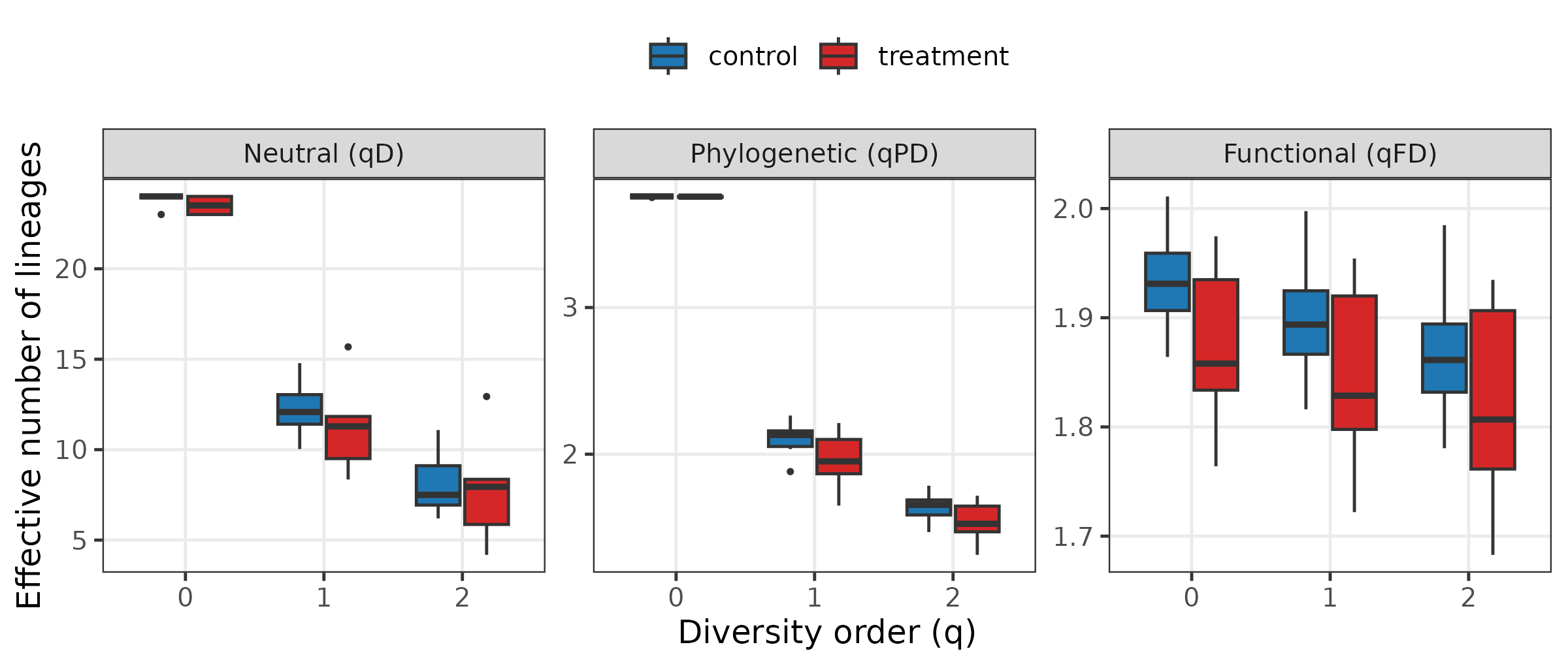

At the alpha (within-sample) level the two groups look almost identical in every flavour: a single host carries about the same number of effective MAGs, spread over about the same amount of the phylogeny and the same functional space, whether or not it received the treatment. Read at the alpha level alone, the intervention looks like it did nothing. The effect is not in how much diversity each gut holds, but in which lineages hold it — a compositional change that only between-sample analysis can see.

Where does the community turn over — and where doesn’t it?

hillpart() partitions diversity between the two groups and reports beta, the effective number of distinct communities. Running it for each flavour shows which axis the treatment shifts:

part <- function(type, ...) {
  m <- as_df(hillpart(gut_counts, q = c(0, 1, 2), hierarchy = ~ group,
                      metadata = metadata, ...))
  m <- m[m$scale == "total", c("q", "beta")]
  m$flavour <- type
  m
}
beta <- rbind(part("Neutral"),
              part("Phylogenetic", tree = gut_tree),
              part("Functional",   dist = fdist))
beta$flavour <- factor(beta$flavour, c("Neutral", "Phylogenetic", "Functional"))

ggplot(beta, aes(factor(q), beta, fill = flavour)) +
  geom_col(position = position_dodge(0.8), width = 0.7) +
  geom_hline(yintercept = 1, linetype = 2, colour = "grey40") +
  scale_fill_brewer(palette = "Set2", name = NULL) +
  labs(x = "Diversity order (q)",
       y = expression("Between-group turnover (" * beta * ")"))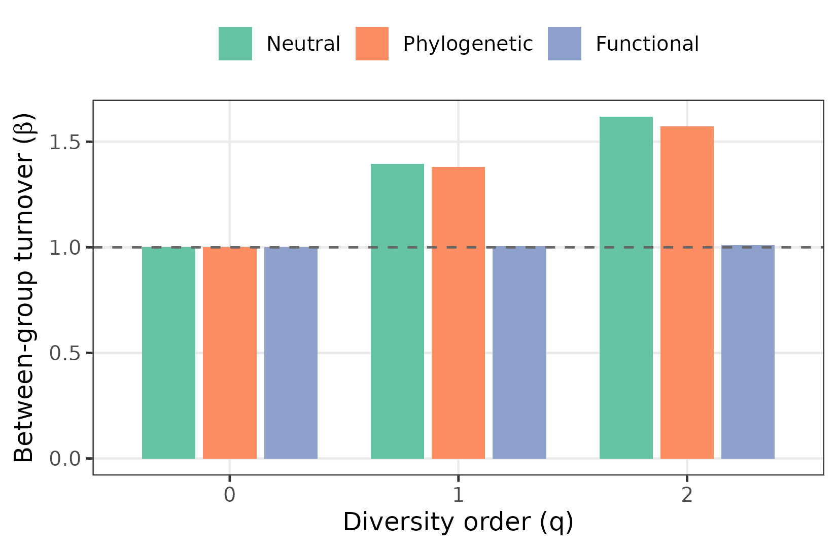

Between-group beta grows strongly with q for the neutral and phylogenetic decompositions but stays essentially flat (β ≈ 1) for the functional one. The clade swap replaces the dominant genomes with phylogenetically distant ones, so taxonomic and evolutionary composition turn over almost in lock-step — yet because the two clades are functional mirrors, the functional make-up of the community barely moves. Distinguishing taxonomic, phylogenetic and functional turnover on one common beta scale is a core strength of the Hill-number framework as implemented here, and here it isolates a change that is phylogenetic but not functional.

Ordination in three spaces

hillpair() accepts the same tree = / dist = switch, so one workflow produces ordinations in neutral, phylogenetic and functional space:

ord_one <- function(d, lab) {
  pc <- cmdscale(d, k = 2)
  o  <- data.frame(pc, mag = rownames(pc))
  names(o)[1:2] <- c("PCoA1", "PCoA2")
  o$group <- grp(o$mag); o$space <- lab
  o
}
ord <- rbind(
  ord_one(hillpair(gut_counts, q = 1, metric = "C"),                 "Neutral (q = 1)"),
  ord_one(hillpair(gut_counts, q = 1, metric = "C", tree = gut_tree), "Phylogenetic (q = 1)"),
  ord_one(hillpair(gut_counts, q = 1, metric = "C", dist = fdist),   "Functional (q = 1)")
)
ord$space <- factor(ord$space,
                    c("Neutral (q = 1)", "Phylogenetic (q = 1)", "Functional (q = 1)"))

ggplot(ord, aes(PCoA1, PCoA2, colour = group)) +
  geom_point(size = 2.4) +
  stat_ellipse(level = 0.68) +
  facet_wrap(~ space, scales = "free") +
  scale_colour_manual(values = pal, name = NULL) +
  labs(x = "PCoA 1", y = "PCoA 2")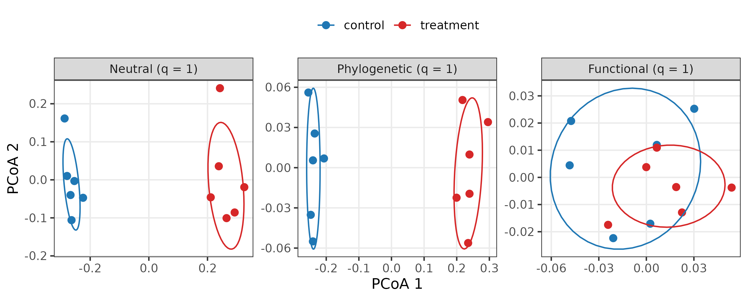

The same samples separate cleanly into control and treatment in neutral space and in phylogenetic space, but collapse onto a single overlapping cloud in functional space. The picture the three panels paint together — who and which lineage differ, what they do does not — is one no single distance could give.

Functional redundancy

hillred() quantifies the functional redundancy that underlies this pattern: it fits the saturating relationship between neutral diversity (number of genomes) and functional diversity (number of distinct trait profiles) across samples. A curve that plateaus well below the spread of neutral diversity means many genomes share functions — so the community can replace genomes without losing function.

red <- hillred(gut_counts, q = c(1, 2), dist = fdist)
as_df(red)[, c("q", "redundancy")]
#>   q redundancy
#> 1 1  0.6957595
#> 2 2  0.6024721
plot(red)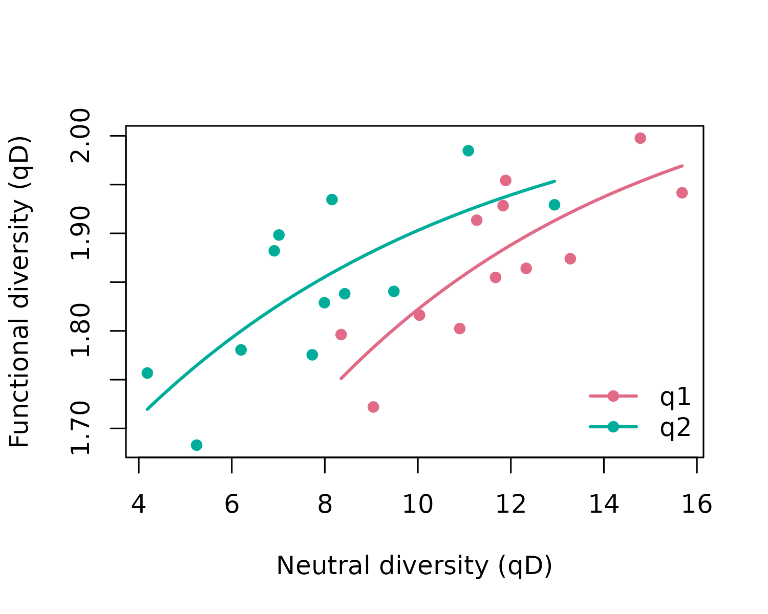

The fitted redundancy is high (around 0.6–0.7): functional diversity saturates well below the spread of neutral diversity, so adding genomes contributes far less than proportional new function. This is exactly why the treatment could overturn the community’s taxonomic and phylogenetic composition without touching its function — every functional role lost with clade A is recovered from its mirror in clade B. The redundancy that hillred() measures is the mechanism the beta and ordination analyses revealed.

Summary

From one MAG table plus a genome tree and a trait table, hilldiv3 produced a complete three-flavour analysis through one interface: trait-to-distance conversion (traits2dist()); neutral, phylogenetic and functional alpha diversity (hilldiv()); between-group partitioning for each flavour (hillpart()); ordinations in neutral, phylogenetic and functional space (hillpair()); and functional redundancy (hillred()). The unified, type-switching interface is what lets a single study separate a change that is taxonomic and phylogenetic from one that is functional — here revealing a community reorganised in identity but conserved in function.

References

• Jost, L. (2007). Partitioning diversity into independent alpha and beta components. Ecology, 88, 2427–2439.
• Chiu, C.-H., Jost, L. & Chao, A. (2014). Phylogenetic beta diversity, similarity, and differentiation measures based on Hill numbers. Ecological Monographs, 84, 21–44.
• Alberdi, A. & Gilbert, M.T.P. (2019). A guide to the application of Hill numbers to DNA-based diversity analyses. Mol. Ecol. Resour., 19, 804–817. ```