Hill numbers computation

Compute neutral, phylogenetic and/or functional Hill numbers (alpha diversity) from a single sample or a count table. By default the computation is cumulative: every diversity type whose inputs are present is returned. Counts are always available, so neutral is always computed; a tree adds phylogenetic and a dist adds functional. Supplying both a tree and a dist therefore returns neutral, phylogenetic and functional side by side in a single tibble (with a type column). Use type to restrict the output to a subset.

Usage

hilldiv(
  data,
  q = c(0, 1, 2),
  tree = NULL,
  dist = NULL,
  tau = NULL,
  type = c("auto", "neutral", "phylogenetic", "functional"),
  reference = c("pool", "sample"),
  out = c("tibble", "matrix")
)

Arguments

data

Counts: a numeric vector (one sample), a matrix/data.frame (taxa x samples), a phyloseq object or a TreeSummarizedExperiment.

q

Numeric vector of diversity orders (>= 0). Defaults to c(0, 1, 2) (richness, Shannon, Simpson).

tree

A phylogenetic tree of class phylo whose tip labels match the taxa in data.

dist

A functional distance matrix (or dist) over the taxa.

tau

Optional functional distance threshold. Defaults to max(dist).

type

Diversity type(s) to compute. "auto" (default) returns every type whose inputs are present (always neutral, plus phylogenetic with a tree and functional with a dist). Pass an explicit type, or a character vector of types, to restrict the output – e.g. "neutral" ignores any tree/dist carried by the object, and c("neutral", "phylogenetic") drops functional even when a dist is supplied. A requested type that lacks its input (e.g. "phylogenetic" without a tree) is an error.

reference

Reference tree depth for phylogenetic Hill numbers (ignored for neutral and functional types). "pool" (default) reads every sample at one common depth T = mean(T_j), so values share a comparable axis across samples; "sample" reads each sample at its own depth T_j (effective lineages at that sample's depth). The two coincide on ultrametric trees. This reference depth is intentionally not offered by hillpart(): in a partition T is fixed at the mean per-sample depth of Chiu et al. (2014), the unique value for which gamma / alpha is a valid decomposition with beta in [1, N].

out

Output shape: "tibble" (default) returns a long-format data.frame with columns q, sample, value (plus a type column when more than one type is computed) and print()/plot() methods; "matrix" returns a matrix with samples in rows and diversity orders (q0, q1, ...) in columns, or, when more than one type is computed, a named list of such matrices (one per type).

Value

A long-format data.frame of class hill_diversity (default). With out = "matrix", a matrix of Hill numbers (samples in rows, diversity orders q0, q1, ... in columns) for a single type, or a named list of such matrices when several types are computed.

References

Chao, A., Chiu, C.-H. & Jost, L. (2010). Phylogenetic diversity measures based on Hill numbers. Phil. Trans. R. Soc. B, 365, 3599-3609.

Alberdi, A. & Gilbert, M.T.P. (2019). A guide to the application of Hill numbers to DNA-based diversity analyses. Mol. Ecol. Resour., 19, 804-817.

See also

hillpart(), hilldiss(), hillprof()

Examples

counts <- matrix(c(10, 0, 5, 2, 8, 1), nrow = 3,
                 dimnames = list(c("t1", "t2", "t3"), c("s1", "s2")))
hilldiv(counts)
#> Computing "neutral" Hill numbers of "q0", "q1", and "q2".
#> ℹ 3 taxa across 2 samples.
#> <hilldiv3 result: neutral>
#> 6 rows x 3 cols
#> 
#>   q sample    value
#> 1 0     s1 2.000000
#> 2 1     s1 1.889882
#> 3 2     s1 1.800000
#> 4 0     s2 3.000000
#> 5 1     s2 2.137309
#> 6 2     s2 1.753623
hilldiv(counts, q = c(0, 1, 2))
#> Computing "neutral" Hill numbers of "q0", "q1", and "q2".
#> ℹ 3 taxa across 2 samples.
#> <hilldiv3 result: neutral>
#> 6 rows x 3 cols
#> 
#>   q sample    value
#> 1 0     s1 2.000000
#> 2 1     s1 1.889882
#> 3 2     s1 1.800000
#> 4 0     s2 3.000000
#> 5 1     s2 2.137309
#> 6 2     s2 1.753623
plot(hilldiv(counts, q = c(0, 1, 2)))
#> Computing "neutral" Hill numbers of "q0", "q1", and "q2".
#> ℹ 3 taxa across 2 samples.


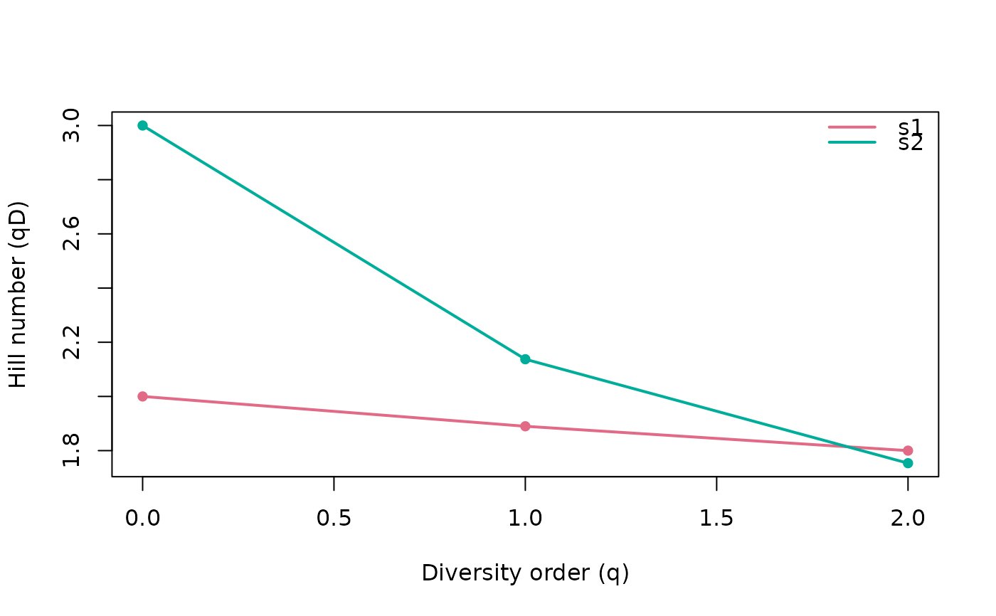# Supplying both a tree and a distance matrix returns neutral, phylogenetic
# and functional diversity together, distinguished by a `type` column.
tree <- ape::read.tree(text = "((t1:1,t2:1):1,t3:2);")
dist <- as.matrix(stats::dist(c(t1 = 0, t2 = 1, t3 = 4)))
hilldiv(counts, tree = tree, dist = dist)
#> Computing "neutral", "phylogenetic", and "functional" Hill numbers of "q0",
#> "q1", and "q2".
#> ℹ 3 taxa across 2 samples.
#> <hilldiv3 result: neutral, phylogenetic, functional>
#> 18 rows x 4 cols
#> 
#>    q sample         type    value
#> 1  0     s1      neutral 2.000000
#> 2  1     s1      neutral 1.889882
#> 3  2     s1      neutral 1.800000
#> 4  0     s2      neutral 3.000000
#> 5  1     s2      neutral 2.137309
#> 6  2     s2      neutral 1.753623
#> 7  0     s1 phylogenetic 2.000000
#> 8  1     s1 phylogenetic 1.889882
#> 9  2     s1 phylogenetic 1.800000
#> 10 0     s2 phylogenetic 2.500000
#> 11 1     s2 phylogenetic 1.702490
#> 12 2     s2 phylogenetic 1.423529
#> 13 0     s1   functional 2.000000
#> 14 1     s1   functional 1.889882
#> 15 2     s1   functional 1.800000
#> 16 0     s2   functional 1.403846
#> 17 1     s2   functional 1.301798
#> 18 2     s2   functional 1.247423

# Restrict the output with `type` (a scalar or a vector):
hilldiv(counts, tree = tree, dist = dist, type = c("neutral", "functional"))
#> Computing "neutral" and "functional" Hill numbers of "q0", "q1", and "q2".
#> ℹ 3 taxa across 2 samples.
#> <hilldiv3 result: neutral, functional>
#> 12 rows x 4 cols
#> 
#>    q sample       type    value
#> 1  0     s1    neutral 2.000000
#> 2  1     s1    neutral 1.889882
#> 3  2     s1    neutral 1.800000
#> 4  0     s2    neutral 3.000000
#> 5  1     s2    neutral 2.137309
#> 6  2     s2    neutral 1.753623
#> 7  0     s1 functional 2.000000
#> 8  1     s1 functional 1.889882
#> 9  2     s1 functional 1.800000
#> 10 0     s2 functional 1.403846
#> 11 1     s2 functional 1.301798
#> 12 2     s2 functional 1.247423